
Recent advances have enabled diffusion models to efficiently compress videos while maintaining high visual quality. By storing only keyframes and using these models to interpolate frames during playback, this method ensures high fidelity with minimal data. The process is adaptive, balancing detail retention and compression ratio, and can be conditioned on lightweight information like text descriptions or edge maps for improved results.
Conditional Diffusion for Video
Let’s test first learn about a diffusion model. A diffusion model generates data by reversing a diffusion process that gradually adds noise to the data unitl it becomes pure noise.
The process is modeled in two phases: the foreard process and the reverse (or backward) process.
Let $x_0 \in \mathbb{R}^d$ be a simple from the data distribution $p_{\text{data}}$.
- Forward Process (Diffusion): This is where we start with data $x_0$ from our desired distribution and add noise over several steps until we get to a point where our data is indistinguishable from noise.
- Reverse Process (Denoising): We learn to reverse the noise addition process. If we do this correctly we can start with noise and apply the reverse process to generate new data sample that appear as if they were drawn from the target data distribution.
Algorithm with code
The process is mathematically decribed using Markov chains with Gaussian transitions.
Forward Transition Kernel:
$q(x_t | x_{t-1}) = \mathcal{N}(x_t; \sqrt{1 - \beta_t}x_{t-1}, \beta_t \mathbf{I})$
At each time step $t$, a Gaussian noise is added to the data. $\beta_t$ is a variance schedule that is chosen beforehand and determines how much noise to add at each step.
Note that we take a square of $\beta$ to scale down $x_{t-1}$ so that after adding noise, the total variance remains 1. It scales down the previous difussed image to make room for the noise and then adding Gaussian noise with just the right variance to maintain the overall variance of the process.
1
2
3
4
5
6
def forward_diffusion(x_0, T):
x_t = x_0
for t in range(1, T+1):
beta_t = beta[t-1]
x_t = np.sqrt(1. - beta_t) * x_t + np.sqrt(beta_t) * np.random.normal(size=x_0.shape)
return x_t
Accumulated Kernel:
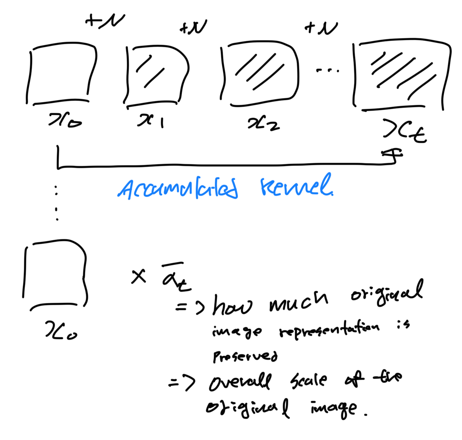
This describes how to sample $x_t$ directly from $x_0$ without going through all intermidate steps.
$q(x_t | x_0) = \mathcal{N}(x_t; \sqrt{\bar{\alpha}_t}x_0, (1 - \bar{\alpha}_t)$

$\bar{\alpha}_t$ is the accumulated product of (1-$\beta_s$) from time 1 to $t$ and represents the overall scale of the original data present in $x_t$.
1 | def sample_from_x0(x_0, t, alpha_bar): |
Reverse Transition Kernel (Reverse Diffusion Process)
The Reverse Diffusion Process (RDP), used to generate new samples from a distribution by reversing the Forward Diffusion Process (FDP). The FDP gradually adds noise to the data, and the RDP aims to learn to reverse this noise addition to recreate the data from the noisy distribution.
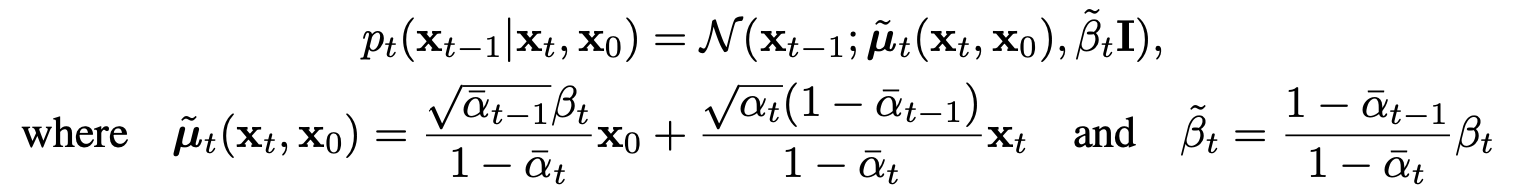
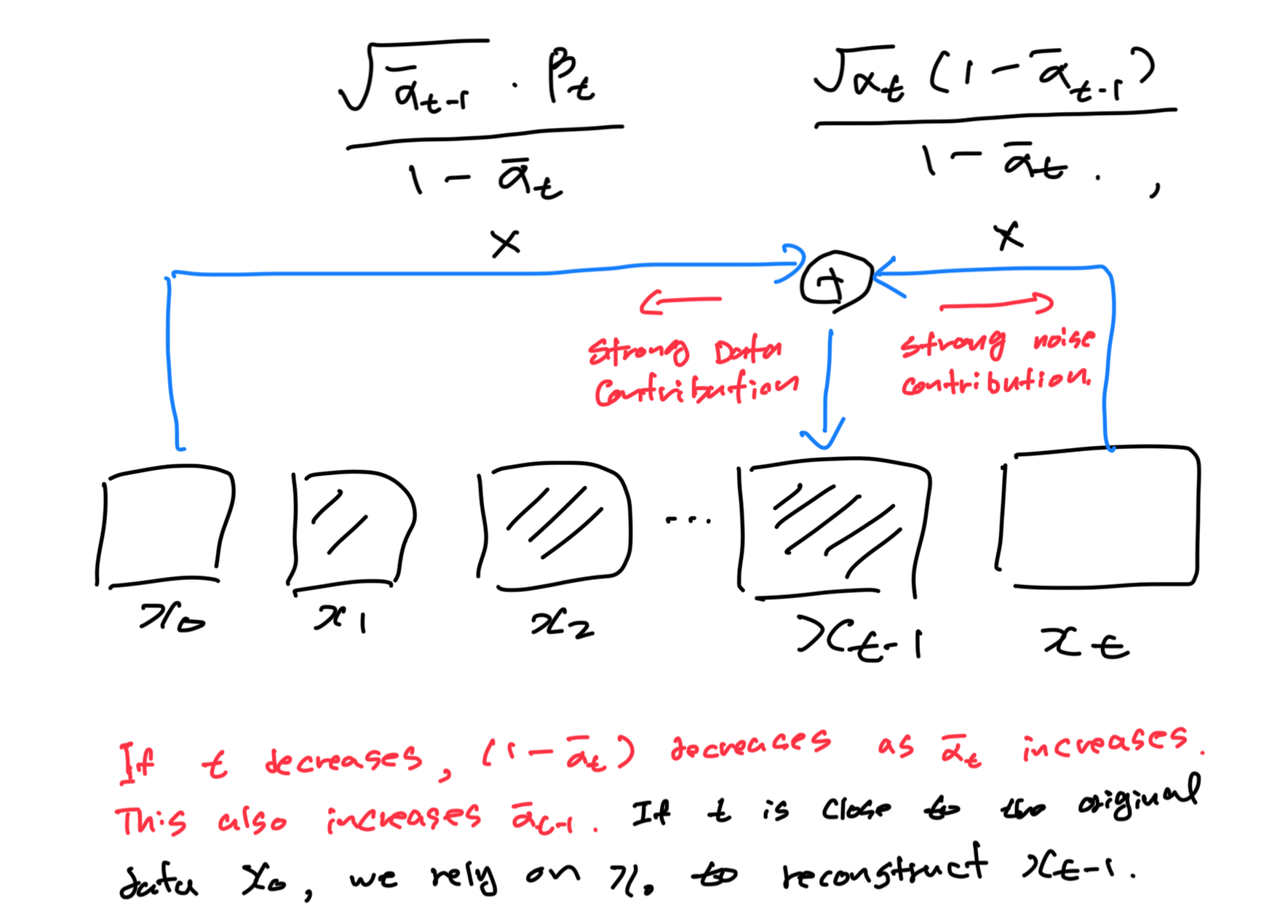
$\tilde{\mu}_t$ is the mean of the reverse transition kernel at time $t$, which is a linear combination of the original data point $x_0$ and the current noisy data point $x_t$.
The $\tilde \beta_t$ term is the variance of the Gaussian distribution for the reverse step, which changes at each step, reflecting how the uncertainty decreases as we approach the original data distribution.
The coefficient for $x_0$ determines how much of the original data point $x_0$ is retained in the reverse transition. As $t$ decreases, $\bar \alpha_{t-1}$ increases, and $1-\bar \alpha_{t-1}$ decreases, making the coefficient larger. This means that as we get closer to $t=0$, we are realying more on the original data point $x_0$ to reconstruct $x_{x-1}$.
The coefficient for $x_t$ determine the contribution of the current noisy data point $x_t$ to the reverse transition. As $t$ decreases, $\alpha_t$ and $\bar \alpha_{t-1}$ is decreases, making the coefficient smaller.
We want to remove just the right amount of noise (represented by $x_t$) while restoring the right amount of signal (represented by $x_0$). Initially, $x_t$ is mostly noisy, so its coefficient is relatively small, but as we reverse the diffusion process, $x_t$ gradually becomes less noisy, and its influence increases.
In the reverse diffusion process, we are effectively using these coefficient to “interploate” between the noise and the data at each step. Initially, the process is noise-dominated, and we have only small “hint” of the data. But as we step back through time, the data’s contribution becomes larger and the noise’s contribution becomes smaller, ultimately allowing us to reconstruct a sample that resembles the original data distribution.
It’s important to note that in practice, $\tilde \mu$ would be predicted by a neural network trained to estimate the denoising step.
With a Neural Network
In a neural network-based approach to reversing the diffusion process to generate data, we focus on estimating the original data $x_0$ from its noisy version $x_t$ without having direct knowledge of $x_0$. This is a critical aspect of the reverse process in diffusion-based generative models.
Estimation of $x_0$:
- Since $x_0$ is unknown during generation, we estimate it from $x_t$, the noisy data at a current timestep.
- The estimation equation $ \hat{x}_0 = \frac{(x_t - \sqrt{1 - \bar{\alpha}_t} \epsilon)}{\sqrt{\bar{\alpha}_t}} $ rearranges the forward process (Equation 2).
- The noise $ \epsilon $ added at each diffusion step is unknown; thus, we utilize a neural network parameterized by $ \theta(x_t | t) $ to estimate this noise.
Neural Network and Loss Function:
- The neural network is defined by its parameters $ \theta $, which are refined during training.
- The loss function $ L(\theta) $ aims to minimize the discrepancy between the estimated noise $ \epsilon $ and the noise predicted by the network $ \theta(x_t | t) $.
- By minimizing this loss, the network is trained to predict the noise added to $ x_0 $ to produce $ x_t $.
Score Function:
- Estimating $ \epsilon $ is tantamount to calculating the scaled gradient of the log density of $ x_t $ with respect to itself, scaled by $ \frac{1}{1 - \bar{\alpha}_t} $.
- This score function denotes the most significant increase direction in the log probability density of the noisy data.
- Simply put, it indicates the direction from the noisy data $ x_t $ towards the original data $ x_0 $.
To delve deeper into the neural network training and the role of the loss function:
- The neural network $ \theta(x_t | t) $ is time-conditional, altering its behavior based on the timestep $ t $, which allows for the accommodation of the varying levels of noise in $ x_t $.
- The loss function $ L(\theta) $ is explicitly designed to make $ \theta(x_t | t) $ an effective estimator of the noise $ \epsilon $ that was incorporated into $ x_0 $ at the time $ t $ during the forward process. Training the network to minimize this loss effectively instructs it on reversing the diffusion process.
- The score function $ \nabla_{x_t} \log q_t(x_t | x_0) $ allows the network’s output to be directly associated with the data’s probability density gradients. This gradient, also known as the score, informs us on adjusting $ x_t $ to enhance its likelihood under the data distribution, which is fundamental to generating representative samples of the original data distribution.
In practice, this methodology enables generative models to create samples from intricate distributions by methodically refining noise into structured data. The neural network is trained to counteract the noise introduced in the diffusion process, thus efficiently generating new data samples from the target distribution.
The entire training process includes the following iterative steps:
- Begin with a sample $ x_0 $ from the true data distribution.
- Introduce noise to generate $ x_t $ following the forward diffusion process.
- Employ the neural network to estimate the noise $ \epsilon $.
- Adjust the neural network parameters $ \theta $ to minimize the disparity between the estimated and the actual noise, in adherence to the loss function.
Upon successful training, the neural network is capable of generating new data samples by initiating from noise and applying the learned reverse process.
References
[1] MCVD: Masked Conditional Video Diffusion for Prediction, Generation, and Interpolation