Ananyzing the ouput of a simulation model is important. How can we be sure that our output is proper and will not hurt an experiment result using those outputs.
Keep this in mind - out is rearely i.i.d. Why do we worry about output? In put processes driving a simulation are random variables. It means our output from the simulation must be random. If we runs the simulation it only yields estimates of measure of system performace, and these estimators are themselves random variables, and are therfore subject to sampling error. Sampling error must be taken into account to make valid inferences concerning system performance.
Measures of Interest
- Means - what is the mean customer waiting time?
- Variances - how much is the waiting time liable to vary?
- Quantiles - what’s the 99% quantile of the line length in a certain queue?
- Sucess probabilities - will my job be completed on time?
- Would like point estimators and confidence intervals for the above.
There are two general types of simulations with respect to output analysis. To facilitate the presentation, we identify two types of simulations with respect to output analysis:
- Finite-Horizon (Terminating) Simulations - Interested in short-term performance
- The termincation of finite-horizon simulation takes place at a specific time or is caused by the occurrence of a specific event.
- EX1 - Mass transit system during rush hour
- EX2 - Distribution system over one month
- Steady-State simulations - Interested in long-term performance
- The purpose of steady-state simulation is to study the long-run behavior of a system. A performance measure is a steady-state parameter if it is a characteristic of the equilibrium distribution of an output process.
- EX1 - Continuously operating communication system where the objective is the computation of the mean delay of a packet in the long run
- EX2 - Distribution system over a long period of time
- EX3 - Markov chains
Finite-Horizon Simulation
First thing we have to do to conduct this simulation is getting expected values from replications. So basically, we need to decide a number of independetn replications (IR). IR estimates Var($\bar{Y}_m$) by conducting $r$ independent simulation runs (replications) of the system under study, where each replication consists of $m$ observations. It is easy to make the replications independent - just re-initialize each replication with a different pseudo-random number seed Sample means from replication
If each run is started under the same operating conditions (e.g., all queues empty and idle), then the replication sample means $Z_1, Z_2, . . . , Z_r$ are $i.i.d.$ random variables.


Suppose we want to estimate the expected average waiting time for the first m = 5000 customers at the bank. We make r = 5 independent replications of the system, each initialized empty and
idle and consisting of 5000 waiting times. The resulting replicate means are:


Steady-state simulation
How about we need to simulate the entire time line? We should consider to use a steady-state simulation. Estimate some parameter of interest, e.g., the mean customer waiting time or the expected profit produced by a certain factory configuration. In particular, suppose the mean of this output is the unknown quantity $\mu$. We’ll use the sample mean $\bar{Y}_n$ to estimate $\mu$
We must accompany the value of any point extimator with a measure of its variance. In stead of Var($\bar{Y}_n)$ we canestimate the variance parameter,
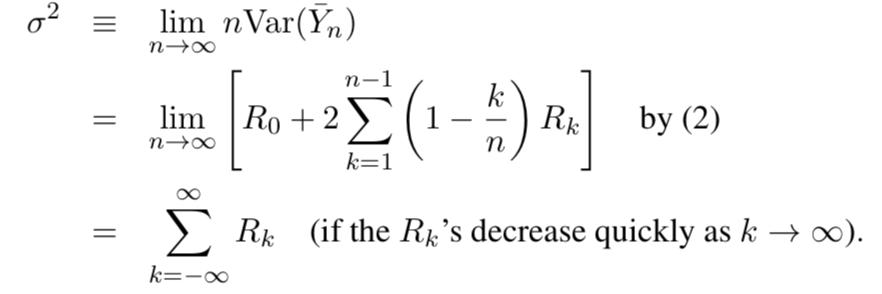
Thus, $\sigma^2$ is imply the sume of all covariances! $\sigma^2$ pops up all over the place: simulation output analysis, Brownian motions, fnancial engineering application, etc.

Many methods for estimating $\sigma^2$ and for conducting steady-state output analysis in general:
Batch means
The method of batch means (BM) is often used to estimate $\sigma^2$ and to calculate confidence intervals for $\mu$
Idea: Divide one long simulation run into a number of contiguous batches, and then appeal to a central limit theorem to assume that the resulting batch sample means are approximately i.i.d. normal.
In particular, suppose that we partition $Y_1, Y_2, . . . , Y_n$ into $b$ nonoverlapping, contiguous batches, each consisting of $m$ observations (assume that $n = bm$)
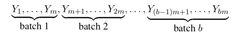
The $i$th batch mean is the sample mean of the $m$ observations from batch $i = 1, 2, . . . , b$


$E[H]$ decreases in b, though it smooths out around b = 30. A common recommendation is to take b =. 30 and concentrate on increasing the batch size m as much as possible.
The technique of BM is intuitively appealing and easy to understand.
But problems can come up if the Yj ’s are not stationary (e.g., if significant initialization bias is present), if the batch means are not normal, or if the batch means are not independent.
If any of these assumption violations exist, poor confidence interval coverage may result — unbeknownst to the analyst.
To ameliorate the initialization bias problem, the user can truncate some of the data or make a long run
In addition, the lack of independence or normality of the batch means can be countered by increasing the batch size m.


Reference
Thumnail
Georgia Tech’s ISYE6644 class content