How can we tell our random variables are well made? In simulation terminology, we have something called input analysis.
In my previous two postings, random number, random variable, I’ve talked about how to generate a random number and how we could make a radom variable by using those random numbers. Then how can we tell our random variables are well made? In simulation terminology, we have something called input analysis. The random variables are our input, and we need to analyze those inputs to verify it’s relevance. If you use the wrong input random variables in the simulation model, it will result in wrong output. A proper input analysis can save you from Garbage-in-garbage-out
How can we conduct a proper input analysis?
- We have to collect data
- Data Sampling - we could shuffle the data and take some samples from there
- We have to figure out a distribution of data
- Plot the data to histogram
- Discrete vs contunuous
- Univariate / Multivariate
- If data is not enough — we can guess a good distribution
- We have to do a statistical test to verify the distribution
1. Point Estimation
A statistic can not explicitly depend on any unknown parameters because statics are based on the actural observations. Statistics are random variable - we could expect to have two different values of a static when we take two different samples. But we need to find the unknown parameters. How can we do it? we could estimate unknown parameters from the existing probability of distribution.
Let $X_1, . . . . , X_n$ be i.i.d. Random Variables and let $M(X) ≡ M(X_1, . . . . , X_n)$ be a statistic based on the $X_i$’s. Suppose we use $M(X)$ to estimate some unknown parameter $θ$ Then $M(X)$ is called a point estimator for $θ$ .
- $\bar{x}$ is a point estimator for the mean $μ = E[Xi]$
- $S^2$ is a point estimator for the variance $σ2 = Var(Xi) $
*It would be nice if $M(X)$ had certain properties: *
- Its expected value should equal the parameter it’s trying to estimate
- It should have low variance
We all know that good estimator should be unbiased because if we use the biased estimator we won’t figure out whether our model is good or not. We will be fooled by a biased estimator. $T(X)$ is unbiased for $θ$ if $E[M(X)] = θ$
EX1 - Suppose $X_1, . . . , X_n$ are i.i.d. anything with mean μ. Then
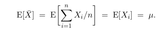
So $\bar{X}$ is alwys unbiased for $\mu$. That’s why ${\bar{X}}$ is called the sample mean
EX2 - Suppose $X_1, . . . , X_n$ are i.i.d. anything with mean μ and variance $\sigma^2$. Then
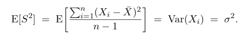
Thus, $S^2$ is always unbiased for $\sigma^2$. This is why $S^2$ is called the sample variance.
2. Mean Square Error
In a perfect sceanario, our estimator will be exactly same as $\theta$. Then we will see no error. However, it’s not the real case. Our goal is to reduce the error between an estimator and $\theta$.
The mean squared error of an estimator $M(X)$ of $\theta$ is
$$
\begin{aligned}
MSE(M(X)) ≡ E[(M(X)-\theta)^2]
\end{aligned}
$$
$$
\begin{aligned}
Baia(M(X)) ≡ E[T(X) - \theta]
\end{aligned}
$$
We could interpret MSE like this:
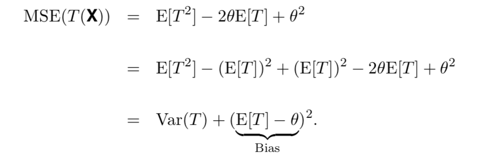
Lower MSE mean we are avoiding the bias and variance. Our goal should be finding a good estimator which can lower our error. If $M_1(X)$ and $M_2(X)$ are two estimators of $\theta$, we’d usually prefer the one with the lower MSE — even if it happens to have higer bias.
3. Maximum Linelihood Estimators
What if we don’t have a set of data, but we have a pdf/pmf $f(x)$ of the distribution. How can we find the $\theta$?
Consider an i.i.d. random sample $X_1, . . . , X_n$, where each $X_i$ has pdf/pmf $f(x)$. Further, suppose that $\theta$ is some unknown parameter from $X_i$. The likelihood function is $L(\theta) ≡ \prod f(x_i)$
The maximum likelihood estimator (MLE) of $\theta$ is the value of $\theta$ that maximizes $L(\theta)$. The MLE is a function of the $X_i$’s and is a RV.
EX1 - Suppose $X_1, . . . , X_n$ ~ Exp$(\gamma)$. Find the MLE for $\gamma$
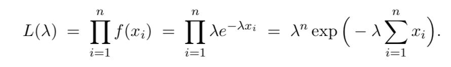
Since the natural log function is one-to-one, it’s easy to see that the $\gamma$ that maximizes $L(\gamma)$ also maximize $ln(L(\gamma))$
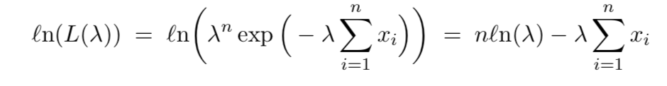
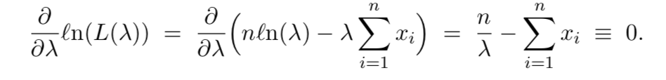
This implies that the MLE is $\hat{\gamma} = 1 / \bar{X}$
Invariance Property
If $\hat{\theta}$ is the MLE of some parameter $\theta$ and $h(.)$ is a one-to-one function, then $h(\hat{\theta})$ is the MLE of $h(\theta)$
For Bern(p) distribution the MLE of $p$ is $\hat{p}=\bar{X}$ (which also happens to be unbiased). If we consider the 1:1 function $h(\theta) = \theta^2$ for ($\theta > 0)$, then the Invariance property says that the MLE of $p^2$ is $\bar{X}^2$
But such a property does not hold for unbiasedness
$$
\begin{aligned}
E[S^2] = σ^2
\end{aligned}
but
\begin{aligned}
E[\sqrt{S^2}]= σ
\end{aligned}
$$
Really that MLE for $\sigma^2$ is $\hat{\sigma^2} = 1/n\sum(X_i - \bar{X})^2$. The good news is that we can still get the MLE for $\sigma$. If we consider the 1:1 function $h(\theta) = +\sqrt{\theta}$, then the invariance property says that the MLE of $\sigma$ is
$$
\begin{aligned}
\hat{\sigma} = \sqrt{\hat{\sigma^2}} = \sqrt{\sum(X_i-\bar{X})^2/n}
\end{aligned}
$$
4. The Method of Moments
Recall: the $k$th moment of a random variable X is
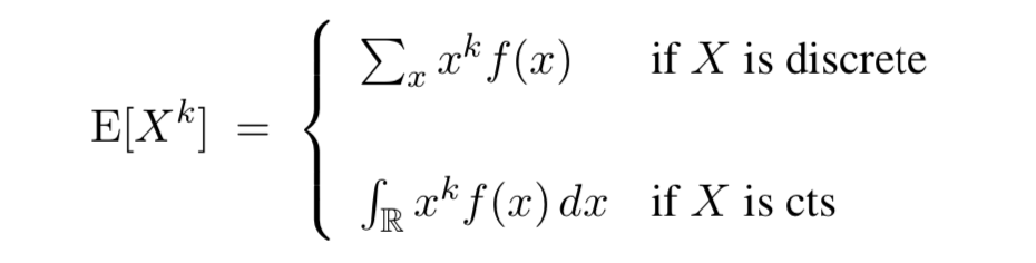
Suppose $X_1, . . . , X_n$ are i.i.d. from p.m.f. / p.d.f. $f(x)$. Then the method of moments(MOM) estimator for $E[X^k]$ is
$$
m_k ≡ 1/n\sum X^k_i
$$

5. Goodness-of-Fit Tests
We finanlly guessed a reasonable distribution and then estimated the relevant parameters. Now let’s conduct a formal test to see just how sucessful our toils have been.
In particular, test
$$
H_0 : X_1, X_2, . . . , X_n - p.m.f / p.d.f. f(x)
$$
At level of significance
$$
\alpha ≡ P(Reject H_0 | H_0 true) =P(\text{Type I Error})
$$
Chi-Square-Test
Goodness-of-fit test procedure:
- Divide the domain of $f(x)$ into $k$ sets, say, $A_1, A_2, A_3, . . . , A_k$ (distinct points if X is discret r intervals if X is continuous)
- Tally the actual number of observations that fall in ach set, say, $O_i i = 1, 2, . . . , k$. If $p_i ≡ P(X ∈ Ai)$, then $O_i \text{~ Bin(}n,p_i)$
- Determine the expected number of observations that would fall in each set if $H_0$ were true, say, $E_i = E[O-I] = np_i, i = 1,2, . . . , k$
- Calculate a test statistic based on the differences between the $E_i$ and $O_i$.
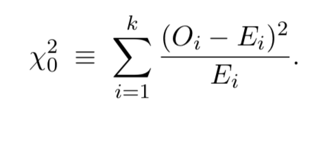
- A large value of $X^2_0$ indicate a bad fit. We reject $H_0 \text{ if } \chi^2_0 > \chi^2_{\alpha,k-1-s}$, where $s$ is the number of nuknown paramets from $f(x) that have to be estimated.
Usual recommendation: For the $\chi^2$ g-o-f test to work, pick $k,n$ such that $E_i >= 5$ and $n$ at least 30
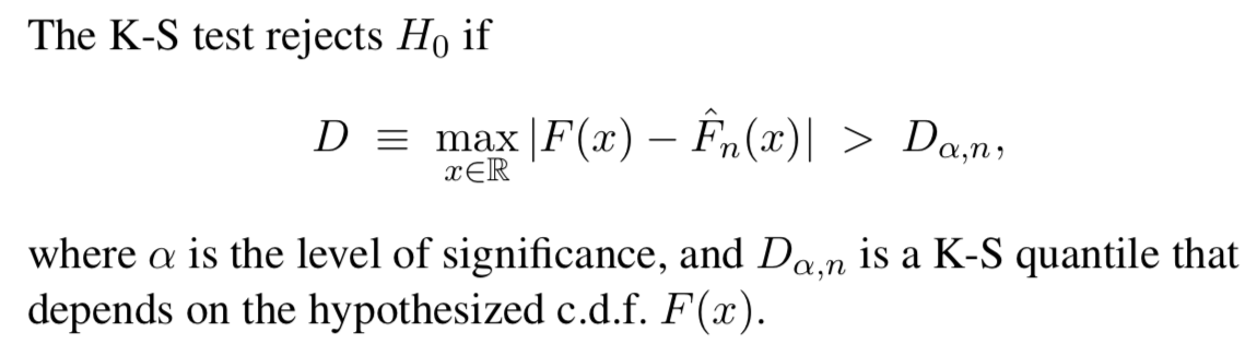
Kolmogorov_Smirnov Goodness-of-Fit Test
We’ll test $H_0 : X_1, X_2, . . . , X_n$ some distribution with $c.d.f. F (x)$.
Recall the difincation of the empirical c.d.f. (also called the sample c.d.f) of the data is
$$
\hat{F_n}(x) ≡ (\text{number of } X_i <= x) / n
$$
The Glivenko-Cantelli Lemma says that $\hat{F_n}(x) -> F(x)$ for all $x$ as $ n->\infinite$. So if $H_0$ is ture then $\hat{F_n}(x)$ should be a good approxmination to the true c.d.f. $F(x)$, for large $n$ The main question: Does the empirical distribution actually support the assumption that H0 is true?
Reference
Thumnail
Georgia Tech’s ISYE6644 class content